
From The Exodus Project
In 1609 Johannes Kepler published his first two laws of planetary motion; the third was published in 1619. In brief, Kepler's Laws are:
Kepler found his laws through a detailed study of the observations of Tycho Brahe, who was perhaps the most precise observational astronomer who has ever lived. Kepler knew that the planets obeyed the laws he had discovered, but he didn't know why they did so. Newton would provide the explanation in his theory of gravity almost 40 years later. We will not - fortunately! - have to derive Kepler's Laws for our purposes. For us, we are interested mainly in his first law: the planets move in ellipses.
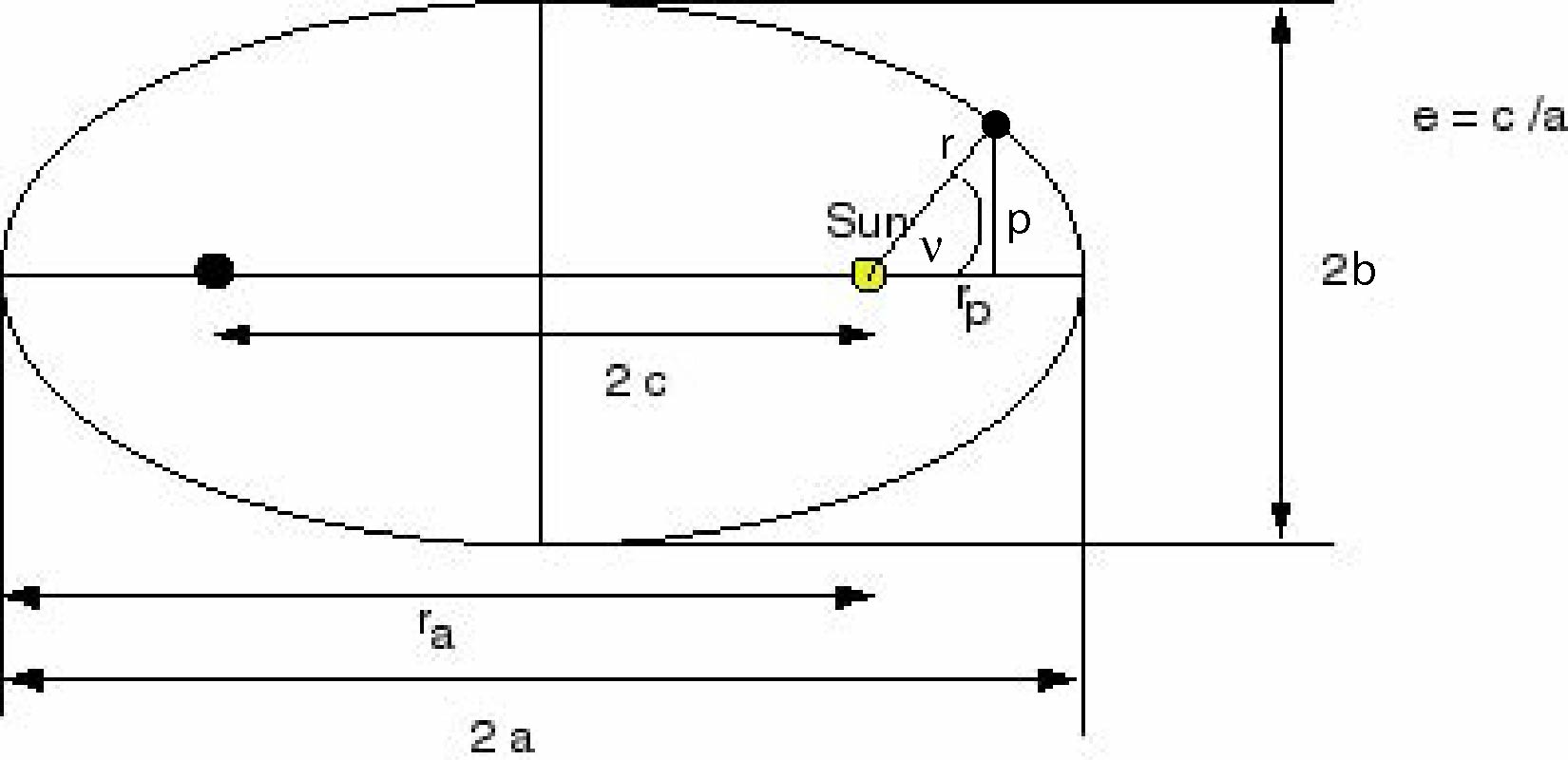
The formula for an ellipse is:
r(DU) = p(DU) / (1+e * Cos[nu(radians)])
where:
nu = 0 corresponds to point of closest approach to the Sun, called the perihelion (rp). nu = pi radians (180 degrees) corresponds to the point where the planet is farthest from the Sun, called the aphelion (ra). One other quantity we will need is the semi-major axis (a), which is half the length of the ellipse. For a circular orbit, this is just the radius of the orbit. It turns out that one needs six parameters, called "orbital elements", to completely define an orbit. We, however, will assume all the planets lie in the same plane (which they don't, but it's a pretty good approximation), so we can ignore some of them. For our purposes, we need only add one more, the longitude of perihelion (Pi). This represents the orientation of the orbit and gives the angle between the orbit's nu=0 line (which passes through perihelion, hence the name) and some arbitrary reference line. For the Solar System, that line is the line between the Sun and the "First Point in Aries", the position of the Earth on the vernal (spring) equinox.
The eccentricity governs the type of orbit. If e=0, then the orbit is circular:
If e is greater than zero but less than one, the orbit is an ellipse:
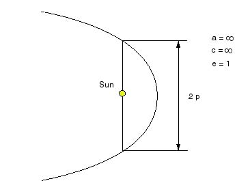
If e=1, the orbit is a parabola:
And finally, if e>1 the orbit is a hyperbola:
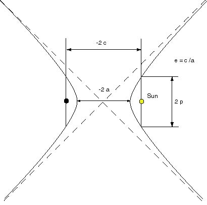
Take a look at the pictures to see what each orbit looks like. Notice that orbits are closed only for e<1. Hyperbolic and parabolic orbits are "escape orbits", achieved only when a body (or a spacecraft) exceeds the escape velocity of the Solar System. Notice also that the semi-major axis of a hyperbolic orbit is negative; check out a good geometry book for the reason why, since it's not really all that important for our purposes.
In general, higher energy is required to reach a higher eccentricity. When a target planet is on the same side of the Sun at arrival as the origin planet was at lDUnch, a hyperbolic orbit is the only possible path and the energy requirements are quite high indeed. A paradox of celestial mechanics is that the least amount of energy is required when the origin and target planets are the greatest distance apart! A circular orbit is the lowest energy orbit, but this orbit is useless to us for orbital transfers becDUse the distance from the Sun is always constant. Related to this, you may be wondering why we can't just fly in a straight line from one planet to another. The reason is that like the planets themselves, our spacecraft is subject to the laws of gravity and therefore to Kepler's Laws. In order to move on a straight line we must have an infinite eccentricity, which requires an infinite amount of energy. Yes, we can travel on a not-too-curved hyperbola, but the energy requirements, as we'll see in the next section, are enormous. For now, however, familiarize yourself with the properties of the four types of orbits, as we will be making extensive use of them in work ahead.
The art of astrogation is essentially the art of placing your spacecraft on an orbit which intersects both your origin planet's orbit and your target planet's orbit (and preferably when the planets in question are at the intersection point!). What, then, determines the orbit of a spacecraft? In a word: energy. The total energy of a spacecraft in orbit is the sum of its kinetic energy (due to its energy of motion in its orbit) and its potential energy (due to the gravitational pull of the Sun). Mathematically, that relationship is:
E(joules/kg) = 1/2 * v(km/s)^2 - mu(km^3/s^2) / r(km)
where:
The gravitational parameter mu is equal to GM, where G is Newton's gravitational constant and M is the mass of the central body. For the Sun, mu = 1.32715 x 10^11 km^3/s^2, but we can make our lives a lot simpler by choosing units such that this constant works out to be 1. It turns out that if we use astronomical units (AU) for our distance unit and 5.0227 x 10^6 sec for our time unit, the gravitational parameter is 1 DU^3/TU^2. The time unit was chosen so that the velocity of the Earth in its orbit is 1 DU/TU. You can convert back to standard units at any time by multiplying times by 5.0227 x 10^6 sec (which is 58.13 days), or by multiplying velocities by 29.79 km/s (the orbital velocity of the Earth). It may seem a bit odd, but it is actually much easier to work in these units.
It can also be shown, however, that for any "conic section" (circle, ellipse, parabola, or hyperbola) the energy is given by:
E(DU^2/TU^2) = - mu(DU^3/TU^2) / (2 a(DU))
where a is the semi-major axis. From this equation we see that a circular or elliptical orbit has negative total energy, which means that the potential energy due to the Sun exceeds the kinetic energy of the spacecraft - the spacecraft is in a "bound" orbit. A hyperbolic orbit has positive total energy and therefore has more kinetic energy than potential energy - the spacecraft will escape from the Solar System. A parabolic orbit has zero energy - the spacecraft will just barely escape, actually only truly being free from the Sun at infinity. Putting this expression for the energy into the original equation gives:
-mu(DU^3/TU^2) / (2 * a(DU)) = 1/2 * v(DU/TU)^2 - mu(DU/TU) / r(DU)
vorb(DU/TU) = Sqrt[2 * mu(DU^3/TU^2) (1 / r(DU) - 1 / (2 * a(DU)))]
For a circular orbit, however, r = a, therefore:
vorb(DU/TU) = Sqrt[mu(DU^3/TU^2) * (2 / r(DU) - 1 / r(DU))] = Sqrt[mu(DU^3/TU^2) / r(DU)]
From looking at this equation you can see that the farther a body is from the Sun, the slower its orbital velocity and the longer it takes to go around the Sun. This is why the orbital periods of the outer planets are so much larger than the orbital periods of the inner planets.
Now, how do we shift between two circular orbits? Obviously a circular transfer orbit won't work - as noted above, we'll always stay at the same radius. As we said at the beginning of this section, what we need is a transfer orbit that will intersect the orbits of both the origin and target planets. In 1925 Hohmann recognized that the minimum energy orbit between two circular orbits is an ellipse which is tangent at the perihelion of one orbit and at the aphelion of the other:
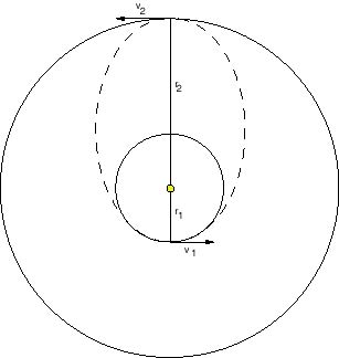
The dashed line represents the transfer orbit and we will assume that we will always launch in the direction of the of the origin planet's orbit so as to take advantage of its orbital energy. Assume that we are launching from the smaller circular orbit. While in orbit with the origin planet, we have a velocity equal to its orbital velocity:
vorb1(DU/TU) = Sqrt[mu(DU^3/TU^2) / r1(DU)]
We need to acquire enough kinetic energy (velocity) to place our spacecraft on the transfer orbit. The semi-major axis of a Hohmann transfer orbit (only, this doesn't apply to other orbits!) is half its length, or:
at(DU) = 1/2 (r1 + r2)
The orbital velocity needed at the insertion point is therefore:
- mu(DU^3/TU^2) / (2 * at(DU)) = 1/2 * v1(DU/TU)^2 - mu(DU^3/TU^2) / r1(DU)
=> v1(DU/TU) = Sqrt[mu(DU^3/TU^2) * (2 / r1(DU) - 1 / at(DU))]
The velocity we need to acquire, the insertion burn, is therefore:
DeltaV1(DU/TU) = v1(DU/TU) - vorb1(DU/TU)
Similarly, the orbital velocity of the larger orbit is:
vorb2(DU/TU) = Sqrt[mu(DU^3/TU^2) / r2(DU)]
and the velocity of the transfer orbit at r2 is:
v2(DU/TU) = Sqrt[mu(DU^3/TU^2) * (2 / r2(DU) - 1 / at(DU))]
And therefore the arrival burn, the velocity needed to go from the transfer orbit to the larger circular orbit is:
DeltaV2(DU/TU) = v2(DU/TU) - vorb2(DU/TU)
The total velocity change needed to make this transfer is therefore:
DeltaV(DU/TU) = DeltaV1(DU/TU) + DeltaV2(DU/TU)
If you refer to the engines article, you can use this value to calculate how much fuel you need to burn to make this transfer. The Hohmann orbit is the lowest possible energy transfer orbit between two circular orbits. It is also the orbit which requires the longest time. The time of flight is just half the period of the orbit, which from Kepler's 3rd Law is:
TOF(TU) = pi Sqrt[mu(DU^3/TU^2) * at(DU)^3]
where at = 1/2 (r1 + r2) and pi (not Pi, the longitude of perihelion from section 1) is 3.1415927.
To calculate a Hohmann transfer orbit between any two circular orbits, follow these steps:
Given the radius of the initial orbit r1 and the destination orbit r2,
Calculate a Hohmann transfer orbit between Earth and Mars (assume both planets are on circular orbits).
Since this is a solar orbit and we take mu=1, then 1 DU = 1 AU and 1 TU = 58.13 days. The orbital radius of the Earth (r1) is 1 AU; the orbital radius of Mars (r2) is 1.524 AU.
Notice that two burns are always required to transfer between orbits. If we omit the second burn, our spacecraft can only perform a flyby maneuver. The second "burn" can be supplied by something other than the spacecraft's engines (aerobraking, gravity capture, etc.), but if we want to remain in the new orbit, some sort of burn is necessary. Also, keep in mind that this procedure applies to any type of orbit: solar, Earth, Lunar, Martian, whatever. Each body has its own value of mu, though we can still set mu=1 and adjust the value of DU and TU.
In general, the planets will not be in the perfect alignment needed for a Hohmann transfer orbit. Suppose we don't want to wait for this arrangement, or suppose we want to arrive sooner than the Hohmann orbit can get us there. To accomplish either of these goals, we need to use a higher-energy transfer orbit. One such orbit is shown below:
Obviously the orbit could also be tangent at none or both of the planetary orbits. If both are tangent, this is just the Hohmann orbit of the previous section. There is usually no reason to use a zero-tangent transfer orbit from a circular orbit, however, as the extra fuel required is rarely justified. The major difference between this orbit and the Hohmann orbit is that the planet and transfer orbital velocities are no longer in the same direction. We must therefore introduce the concept of the "flight path angle", shown as phi1 in the diagram below:
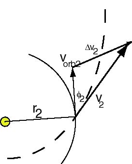
v1, vorb1, and DeltaV1 are found as in the previous section, but the total arrival burn is now found using the law of cosines:
DeltaV2(DU/TU)^2 = v2(DU/TU)^2 + vorb2(DU/TU^2 - 2 *v2(DU/TU) * vorb2(DU/TU) cos[phi2(radians)]
The flight path angle phi2 can be found from the angular momentum of the orbit, which is in turn found from the semi-latus rectum (pt) of the orbit (again, I won't prove this, though it's not difficult to do). That relationship is:
cos[phi2(radians)] = Sqrt[mu(DU^3/TU^2) * pt(DU)] / (r2(DU) * v2(DU/TU))
Putting this into the arrival burn equation gives:
DeltaV2(DU/TU)^2 = v2(DU/TU)^2 + vorb2(DU/TU)^2 - 2 * vorb2(DU/TU) * Sqrt[mu(DU^3/TU^2) *pt(DU)] / r2(DU)
where v2 and vorb2 are found using the formula of the previous section. Now, however, for a transfer orbit tangent at the inner circular orbit (an outbound transfer, as shown in the diagram), the semi-major axis of the transfer orbit is given by.
at(DU) = r1(DU) / (1 - et)
where the transfer orbit eccentricity is found from:
et = pt(DU) / r1(DU) - 1
Both of the expressions can be found from the equation for a conic section. If the transfer orbit is tangent at the outer circular orbit (an inbound transfer), the semi-major axis is given by:
at(DU) = r2(DU) / (1 + et)
and the transfer orbit eccentricity is found from:
et = 1 - pt(DU) / r2(DU)
The total velocity change needed is again:
DeltaV(DU/TU) = DeltaV1(DU/TU) + DeltaV2(DU/TU)
Notice, incidentally, that when the flight path angle is zero, this gives the same relationship found for the Hohmann orbit of the previous section.
Calculating the time of flight is a little trickier, but not terribly difficult. Recall the orbit equation from section 1:
r(DU) = pt(DU) / (1 + et * cos[nu(radians)])
Since we know the eccentricity and semi-latus rectum of the transfer orbit, we can find the true anomaly at the final orbit intercept point using the orbit equation again:
Cos[nu2(radians)] = (pt(DU) / r2(DU) - 1) / et
for an outbound transfer or
Cos[nu2(radians)] = (pt(DU) / r1(DU) - 1) / et
for an inbound transfer.
Keep in mind that the Hohmann orbit is the lowest energy transfer orbit which can reach the target orbit. If, for an outbound transfer, you choose a semi-latus rectum which is smaller than that of the Hohmann orbit (and similarly if you choose a semi-latus rectum which is larger than that of the Hohmann orbit for an inbound transfer), there will be no solution to the problem - the spacecraft doesn't have enough energy to get there at all!
Now, to find the time of flight, we need to use Kepler's Equation. Kepler's Second Law tells us that orbits sweep out equal areas (area being determined by nu) in equal times. This is precisely the relationship we need to find the time of flight along the orbit from nu1 to nu2 . But what, exactlly, is the relationship between the area swept out and nu? The relationship is based on geometrically arguments that we won't go into here, but Kepler found it convenient to introduce an auxillary variable called the eccentric anomaly, or E (which, unfortunately, has the same symbol as the energy of the orbit). Essentially, the eccentric anomaly is the angle from perihelion to a point on a circumscribed circular orbit directly above the position indicated by the true anomaly:
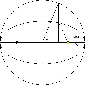
The eccentric anomaly is related to the true anomaly by:
E(radians) = ArcCos[(et + Cos[nu(radians)]) / (1 + et * Cos[nu(radians)])]
E is defined so that it is always in the same half-plane as nu (in other words, when nu is between 0 and pi, so is E). But for an inbound transfer, nu is greater than pi, so E must be in this half-plane as well:
E(radians) = 2 * pi - ArcCos[(et + Cos[nu(radians)]) / (1 + et * Cos[nu(radians)])]
In terms of eccentric anomaly, the time of flight ("Kepler's Equation") is:
TOF(TU) = Sqrt[at(DU)^3 / mu(DU^3/TU^2)] (E(radians) - et * Sin[E(radians)])
Don't forget, however, that this time of flight is from perihelion. But for the inbound transfer we are launching from aphelion not perihelion, so you must subtract off the time required to travel from perielion to aphelion. This time is just half the period of the orbit (which is not coincidentally equal to the Hohmann transfer time). The time of flight equation is therefore:
TOF(TU) = Sqrt[at(DU)^3 / mu(DU^3/TU^2)] (E(radians) - et * Sin[E(radians)]) - pi * Sqrt[mu(DU^3/TU^2) * at(DU)^3]
=> TOF(TU) = Sqrt[at(DU)^3 / mu(DU^3/TU^2)] (E(radians) - et * Sin[E(radians) - pi])
To calculate a one-tangent transfer orbit between any two circular orbits, follow these steps:
Given the radius of the initial orbit r1 and the destination orbit r2, and the semi-latus rectum (the "width") of the transfer orbit pt (NOTE: This must be greater than pt for a Hohmann orbit):
Calculate a one-tangent transfer orbit between Earth and Mars (assume both planets are on circular orbits). Use a semi-latus rectum for the transfer orbit of 1.25 AU (Hohmann pt = 1.21).
Since this is a solar orbit and we take mu=1, then 1 DU = 1 AU and 1 TU = 58.13 days. The orbital radius of the Earth (r1) is 1 AU; the orbital radius of Mars (r2) is 1.524 AU.
So you see that by increasing the total deltaV from 5.66 km/s to 8.60 km/s, our transfer orbit is much more eccentric, allowing us to arrive at Mars earlier (5.89 months instead of 8.63 months).
I have written a Java applet to perform all of these calculations for Solar System orbits, but it is important to keep in mind what you've learn here so that you can properly interpret the results. To use the applet, first select an origin and target planet. The applet will automatically calculate the Hohmann orbit parameters for the two planets you specify. If this is the orbit you want, simply press the "Calculate" button, and the applet will calculate the time of flight and deltaV required for the transfer. If you have specified an engine type, it will also calculate the percentage of your spacecraft that must be fuel in order to make this transfer. If you want a faster transfer, just increase (for an outbound orbit) or decrease (for an inbound orbit) the suggested semi-latus rectum and press the "Calculate" button again. Note that the applet assumes circular planetary orbits - the eccentricity data is presented only for your reference. Have fun!
Article ©2006 Keith Watt
All rights reserved.