
from Graphic Aids In Engineering Computation Randolph P. Hoelscher, Joseph Norman Arnold, and Stanley H. Pierce, (McGrew-Hill Book Company, New York, N.Y.) 1952.
6.1. Utility of Special Slide Rules. By permitting the motion of functional scales along parallel lines the same general types of formulas can be solved as on the straight-scale alignment charts, although the sliding scales have certain inherent limitations not present in some of the straight-scale charts. The special slide rule with parallel moving scales requires no auxiliary index lines and is also more convenient than the alignment chart in being less bulky. The standard slide rule, although adaptable to a great variety of problems, is often not as rapid as a special slide rule developed for a particular problem.
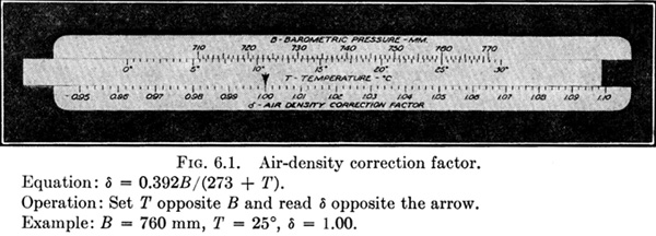
Occasionally, a special slide rule is more accurate than the standard slide rule. As an example, Fig. 6.1 shows a special slide rule for the air-density correction factor represented on a chart in Fig. 3.19. Barometric pressures from 710 to 770 mm are represented on the actual rule by a scale 7 in. long. If an ordinary slide rule having 10-in. scales is used in solving this equation, the entire range from 710 to 770 is contained in a space less than ½ in. in length; thus, at least one more significant figure can be obtained by using the special slide rule. Also, the special slide rule performs the addition of 273 to the temperature, which cannot be done by the ordinary rule.
6.2. Principles of the Parallel-slide Rule. The special slide rule and the ordinary slide rule too, for that matter, operate by adding lengths proportional to the values of the functions represented on their scales.
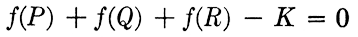
If
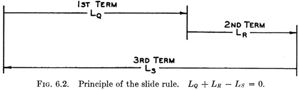
then a slide-rule scale arrangement such as Fig. 6.2 will solve the equation of lengths.

If m is the factor of proportionality, or functional modulus, for all of the scales, then

where f(Q), f(R), and f(S) are any functions of the variables Q, R, and S. Dividing Eq. (2) by m, the relation between the functions is obtained,

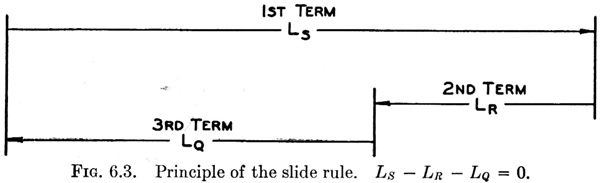
Figure 6.3 is a different arrangement of the same three lengths for which the equation is

or

which is identically the same as Eq. (3) with all signs changed. The geometrical relations for four, five, and six or more functional scales may be obtained in a similar manner.
From this brief explanation of the parallel-slide rule two conclusions may be drawn that are important in the design of special slide rules:
The middle-support rule may later appear to be an exception to these conditions, but the middle-support rule is in reality two slide rules on the same frame, and entirely different moduli may be used on the two halves. Because of the interdependence of the two halves of the middle-support rule, the order of scales is not entirely arbitrary.
6.3. Order and Direction of Scales. It is possible to devise several ways for operating the slide-rule scales to add mechanically the lengths
as shown in Figs. 6.2 and 6.3, but it is desirable that the same general method of operation be used on all special slide rules, and the best method of operation for slide rules without a runner is as follows:
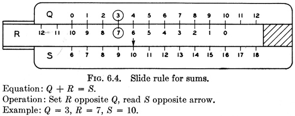
Set the value of the second variable opposite the value of the first, and read the result opposite an index on the lower scale (see Fig. 6.4). This corresponds to the method ordinarily used in performing division on the standard slide rule. In the case of four variables no index is used, and the answer is read on the lower scale opposite the value of the third variable. An example to illustrate this will be shown later.
By means of a simple key the directions of scales for this method of operation may be conveniently obtained as follows:
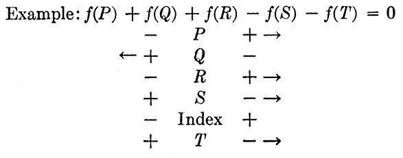
To obtain the order and direction of the scales for the equation

it is first written

then the key is formed
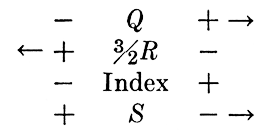
The sign before Q in Eq. (7) is +; so the arrow is placed opposite + in the key. The sign before R is +, but since the signs alternate in the key, R increases to the left. The sign before S is - in Eq. (7), and the
scale increases to the right as shown. The slide rule constructed according to this key is shown in Fig. 6.5. If the position of the index and R scale are interchanged in the key and on the rule, all scales will increase to the right. An inversion of the slide in the frame is the only thing
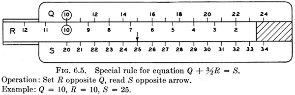
necessary to produce this change. The order and direction of scales for Fig. 6.4 are exactly the same as for Fig. 6.5, and Eq. (7) is different from the equation of Fig. 6.4 only in the coefficient of R. The two slide rules differ only in the range of numbers chosen and in the scale modulus of the R scale, it being 3⁄2 times as much in Fig. 6.5 as in Fig. 6.4.
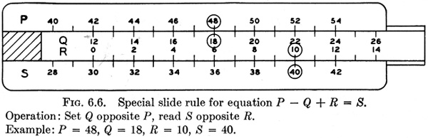
If it is desired to solve

the key becomes
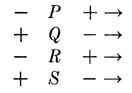
and all scales increase to the right as shown in Fig. 6.6. Because we are accustomed to reading scales which increase to the right, it is desirable to arrange the terms in the equation so that most of their scales will increase to the right. However, it is also desirable that the answer scale (the quantity usually solved for) come at the bottom of the rule. Both
of these points should be considered in selecting the scale arrangement for a practical problem.
From the discussion of Fig. 6.6 it is evident that the index of Fig 6.5 is in reality a scale with but a single point, and that point is for R = 0. Changing the position of the index changes the equation solved on the rule of Fig. 6.5 by an added constant. If the index is moved 2 units to the right, the equation solved by the rule becomes

If the scales for Q, R, and S are replaced by logarithmic scales, Eq. (10) can be solved.

or
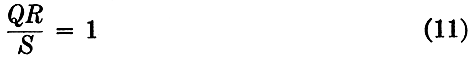
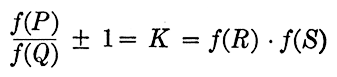
If the index on the slide rule with logarithmic scales is shifted, the equation solved is changed by a constant multiple, so that instead of the constant 1. in Eq. (11) any other constant may occur. Figure 6.7 shows a slide rule having one index for solving the equation QR = S and another index for QR = S/3.

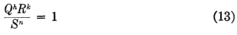
Also of importance is the fact that any coefficients of the logarithmic functions become powers in the product form. For example,
 or
or
6.4. Types of Equations. The following types of equations may be applied to slide-rule blanks of the forms illustrated in the examples.
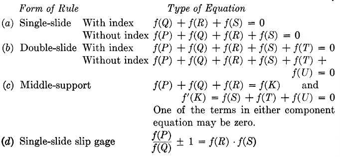
The quantities f(P), f(Q), f(R), f(S), f(T), and f(U) in the type equations above may be any functions of the variables P, Q, R, S, T, and U. The type equations for the single-slide and double-slide rules are in a form for constructing the scales directly; for the middle-support rule the equation is broken into two equations with an auxiliary variable K. For example, if

one half of the middle-support rule is then used to solve
and the other half of the rule solves

The two K scales are placed on opposite sides of the stationary middle support, the corresponding values of K on the two scales are connected
by transfer lines, and the numerical values of K are omitted from the scales.
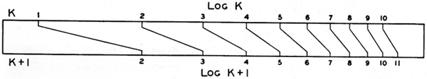
An auxiliary function is also used in designing a slip-gage rule. If
then the two equations solved on the slip-gage rule are

and

Figure 6.8 shows how the scales for log K and log (K + 1) are connected by transfer lines.
The task of transforming an equation into one of the forms given here requires greater ingenuity and is less subject to rules than any other part of the work. The suggestions given in Art. 5.11 may be helpful.
6.5. Enumeration of Steps in Design. A suggested order of attack on a special slide-rule problem is given herewith, considered only from the theoretical point of view. Practical suggestions about marking the scales and pasting them on the blanks are given later.
Step 1. Arrange the equation in proper form for preparing a slide rule. If several of the foregoing forms can be used, choose the one which will be easiest to operate.
Step 2. Arrange the terms in the equation so that the quantity usually solved for comes last and the signs of the terms alternate as nearly as possible.
Step 3. Choose the limits of the variables and select the modulus so that the length of the longest scale will not exceed the length of the slide-rule blank. Functional moduli of all scales must be the same except for a middle-support rule.
Step 4. Determine the directions of increasing values of the functions by arranging the terms in a column in the order in which they are to appear on the rule, and place arrows with reference to the signs as indicated previously.
Sometimes a rearrangement of the scales or a shift in the position of the index will make it possible to have more of the scales increasing to the right.
Step 5. Plot the scales, and paste all of them on the rule; then locate the index by solving an example. If there is no index, the position of one of the scales along its axis must be located by solving an example.
Step 6. The finished slide rule should have all scales clearly labeled with the symbol and units of the quantity represented on them. The date, name of the designer, and a description of the method of operation should also appear on the rule, and it should not be necessary to turn the rule end for end to make data on the back readable.
6.6. Single-slide Rule. The six steps in the design of a single-slide rule shown in Fig. 6.9 will be illustrated with the Column Formula,
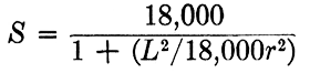
The limits for the variables are L, 1 to 60 ft; r, 0.5 to 5.0 in.; and S 5,600 to 15,000 psi.
Step 1. Write the equation in proper form. First write
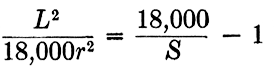
Then by taking logarithms
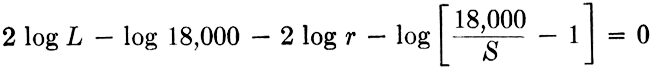
Step 2. Arrange terms in the desired order for use on the slide rule. The form above is satisfactory.
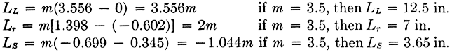
Step 3. Choose the modulus so that with the limits given (or chosen in any problem where not assigned) the length of scale will come within the length of the slide-rule blank, namely, 14 in.
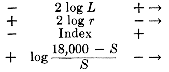
Step 4. Write the key, which indicates that all three functions increase to the right. The function of S is peculiar in that it decreases as S
(* L is in inches in the equation. Changing to feet on the slide rule merely changes the position of the index. )
increases, so that the scale for S has values increasing to the left. The logarithmic functions usually encountered increase as the variable increases, but in this example and in trigonometric scales care must be used to see that the directions of increasing values of the functions are obtained from the key and not necessarily the direction of the increasing value of the variables.
Step 5. When a number of special slide rules are to be constructed, it is a great convenience to have a set of logarithmic scales of various moduli. The chart in the pocket at the back of the book may be used to plot logarithmic scales for moduli between 2.5 and 15 in. In this example the scale modulus for L and r is 2 × 3.5 = 7 in.
For functions other than a constant times the logarithm of the variable, it is usually best to calculate the scale distances for most of the points. For logarithmic scales of a constant plus the variable and for some other forms, the logarithmic chart may sometimes be used. The computations in Table I show how the distances are obtained for plotting the S scale.
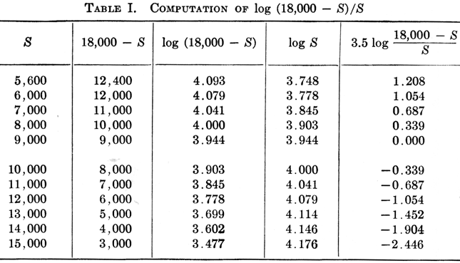
Intermediate values on the plotted scale may be obtained with sufficient accuracy by geometrically dividing the distances between the points computed in the table, or a sector chart may be used. The scale can be plotted both ways from the position selected for S = 9000. The negative sign indicates that the function (18,000 - S)/S has a value less than 1. Although the calculations for the points on the S scale have been carried to more places than can be read on the engineer's scale used in plotting the values, it is better to be too accurate than not accurate enough.
Step 6. The desirability of notes giving the equation, units, and method of operation is obvious. It is also desirable to give any additional information that will make the use of the slide rule more convenient. Ordinarily such notes are placed on the back, but they have been included in the figure title for these examples. A note is added for the Column Formula saying that L/r should not exceed 120 for primary members or 200 for secondary members, and an additional scale shows these two values of L/r.
If the ordinary slide rule is used for this equation, at least three distinct operations of the rule are required besides the mental addition of the constant 1. Obviously this rule will save considerable time in computation, and mistakes are not likely to occur.
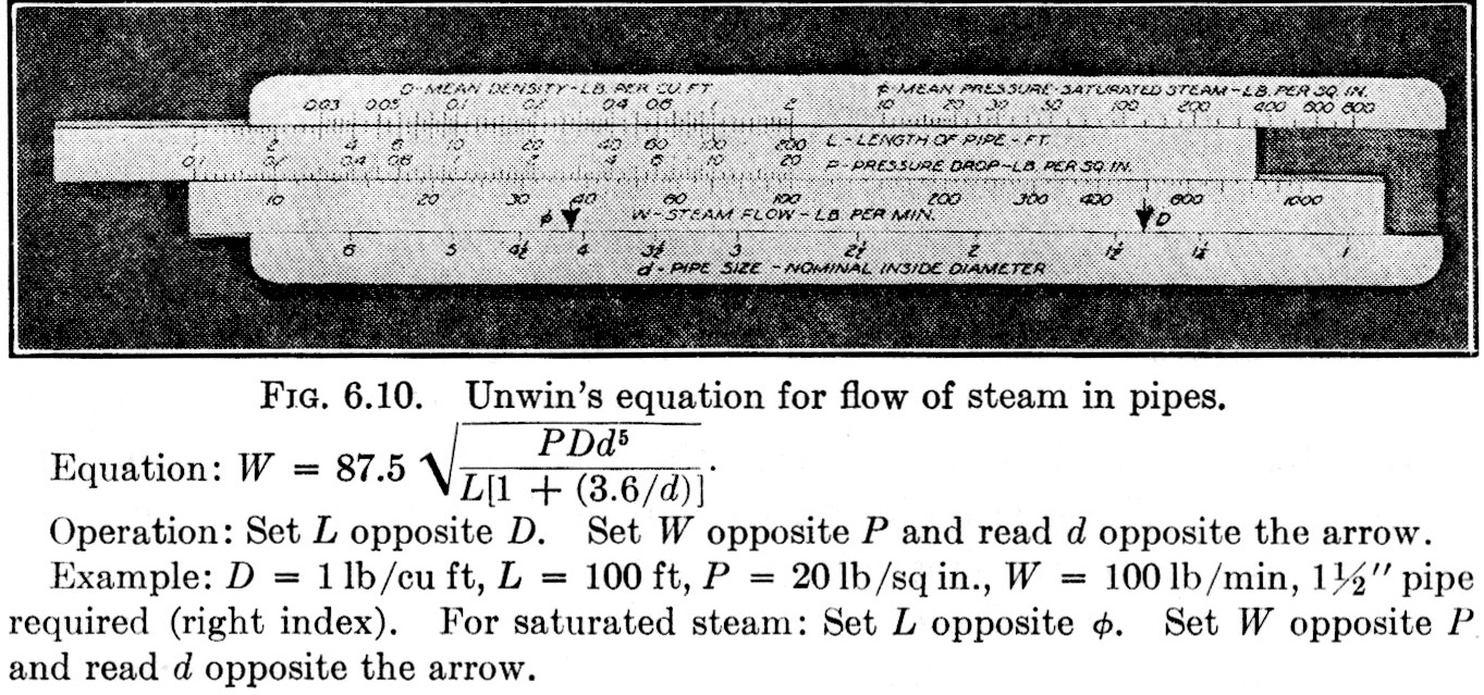
6.7. Double-slide Rule. The construction of this type of rule illustrated by Unwin's equation for the flow of steam in pipes. The equation solved by the special slide rule shown in Fig. 6.10 is
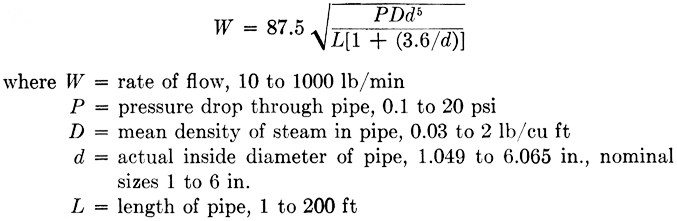
Step 1. The equation reduced to proper form is

Step 2. The equation as written above has the terms in proper order for making a slide rule.
Step 3. Upon the basis of scale lengths shown below the functional modulus was chosen as 3 in.
The other scale lengths are less than 12 in., and the computations have therefore not been shown here. The scale modulus for P, D, and L is 3 in., but for W it is 6 in.
Step 4. The key to determine the direction of the scales is
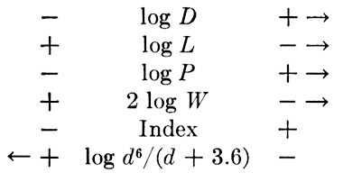
Step 5. All scales except the one for d may be plotted directly with the logarithmic chart at the back of the book. For d, a table of values must be computed and the results plotted. This computation and tabulation have been omitted.
Step 6. The material shown in the figure title should be lettered on the back of the rule.
Solving this equation with the ordinary slide rule is tedious and the results are subject to error because of the complicated function of d. Also, it will be noted that the pipe diameter appearing in the equation is the actual diameter, while pipes are commonly denoted by their nominal diameter. The slide rule has been calibrated in terms of nominal diameters, thus avoiding the necessity for a table of actual and nominal sizes in making computations. The scale for mean pressure, φ (a function of D not shown in the equation), is sometimes convenient for calculations involving saturated steam, but it must not be confused with the pressure drop P. Although all of the scales and arrows are represented in Fig. 6.10 in black, it is desirable to have the φ scale and the corresponding index in red. The φ scale is constructed in the same way as the wire-size scale of Fig. 6.11, using data from steam tables.
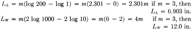
6.8. Middle-support Rule. The equation for transmission-line reactance will be used as an illustration of a middle-support rule shown in Fig. 6.11. The equation is
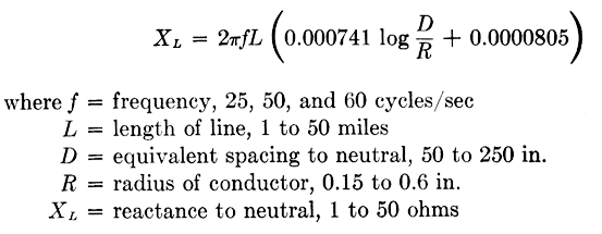
Step 1. The equation is rewritten in proper form
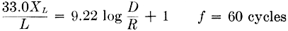
then the auxiliary function
and

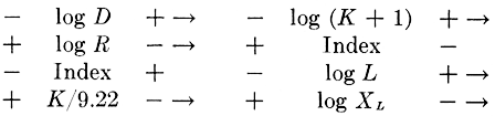
Step 2. The terms are rearranged in the following order so that the top half of the rule solves
and the bottom half solves

Step 3. The functional modulus of all scales on the top half of the rule is 10 in.; on the bottom half it is 7 in.
Step 4. The key must be arranged so that the scales for K and for log (K + 1) increase in the same direction.
Step 5. The index for 60 cycles is located by solving an example. Since the functional modulus of all scales on the lower half of the rule is 7 in., the index marks for 50 cycles and 25 cycles can be found by using the log chart, with a modulus of 7, setting the value 60 on the chart at the index for 60 cycles, and making marks at 50 and 25, respectively.
Step 6. The instructions for operation of the rule, given in the legend for Fig. 6.11, are ordinarily placed on the back of the rule.
The upper index and the frequency scale would ordinarily be omitted until after the scales are affixed to the slide-rule blank; then their location can be accurately determined by solving an example. This slide rule illustrates a device that is often of value; although the radius of conductor, R, appears in the equation, it does not appear on the finished slide-rule scale. The scale for R is marked in terms of wire gage rather than radius, thus making it unnecessary to refer to a wire-gage table in order to use the slide rule.
This method of marking scales in terms of a function other than the one appearing in the equation can also be used advantageously in some aeronautical equations, in equations involving data from a magnetization curve or steam table (φ scale, see Fig. 6.10), and in other cases where the relation between the variable in the equation and the one it is desired to mark on the scale is given by a curve Whose equation may or may not be known.
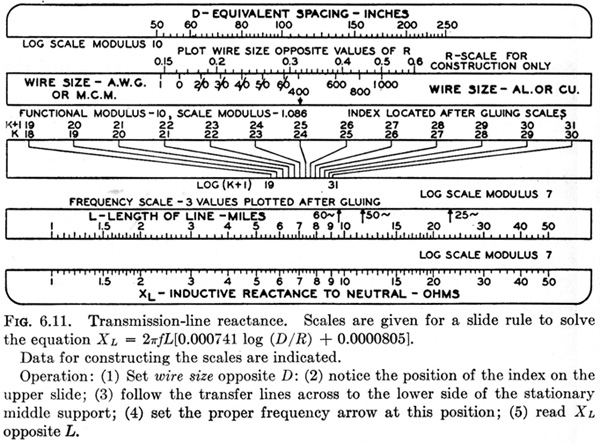
Figure 6.11 shows how this is accomplished. The scale for the function, log R, in the equation is first constructed; then the values of the other variable (wire size in this case) are marked opposite their value in terms of the variable in the equation. The first scale is cut off when the scale strips are prepared and pasted on the slide-rule blank.
As a second illustration, the equation which is used for the special slide rule shown in Fig. 6.12 and which occurs in heating and ventilating is as follows:
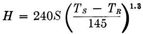
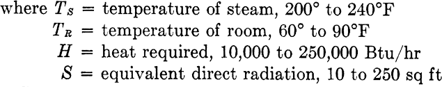
Step 1. Arrange the equation in proper form.
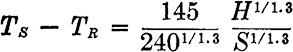
Step 2. Write the equation with the terms in the order in which they
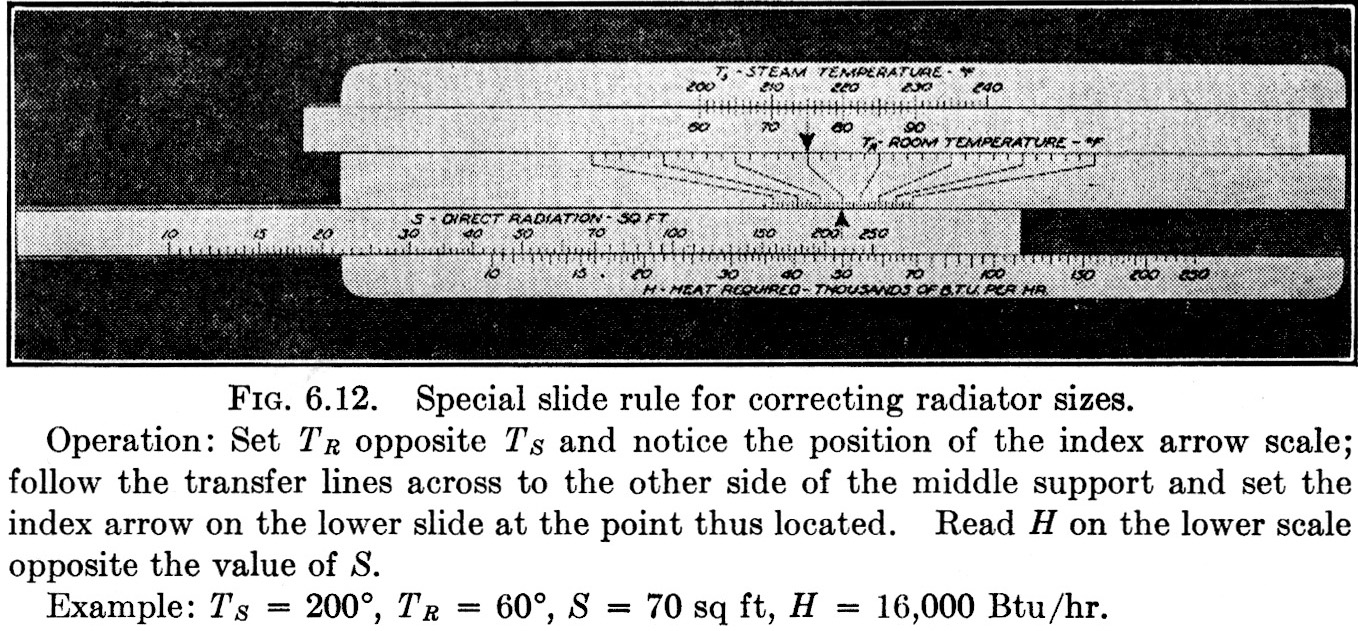
are to appear on the rule. This requires the insertion of an auxiliary term, thus making two equations,
which is solved on the top half of the rule, and

which is solved on the bottom half of the rule.
Step 3. The choice of modulus, construction of the key, and the remainder of the solution are left to the reader.
The features of this slide rule that lead to its inclusion in this group of examples are
1. The exponent 1.3, which makes it awkward to solve the equation with the ordinary slide rule, is conveniently taken care of with the special rule.
2. It shows how equations combining both multiplication and subtraction may be solved with a special slide rule.
3. The equation is used only within the limits, TR between 60 and 90, TS between 200 and 240, and the special slide rule definitely restricts the use of the equation to the proper limits.
There are many other examples of engineering equations which hold throughout only a limited range of the variables and for which a graphical method of solution can be similarly restricted.
6.9. Single-slide Slip-gage Rule. The Francis Weir formula
for the flow of water over a rectangular weir, shown in Fig. 6.13, will be used to illustrate this type of rule. The variables are
Q = quantity of water discharged, 0.1 to 10 cu ft/sec
B = breadth of weir, 1 to 10 ft
H = head of water over weir, 0.5 to 4 ft
Step 1. Write the equation in proper form. It will be observed that both subtraction and multiplication appear in this equation as in the
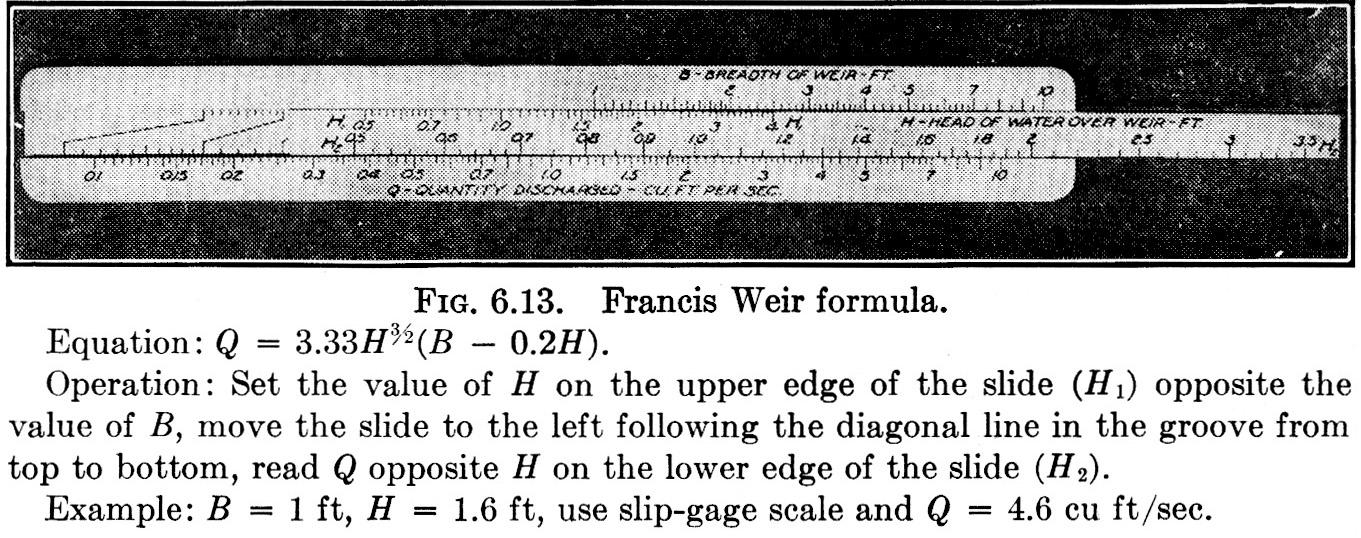
example of Fig. 6.12. An alternate way of preparing a slide rule for such a problem is illustrated in Fig. 6.13, in which the slip-gage scales in the groove subtract the constant 1 from B/0.2H ; that is, the equation is written in the form
and the slide rule first solves B/0.2Hin the usual manner, and then by means of the uncalibrated slip-gage scale in the groove the 1 is subtracted (Figure 6.8 shows the construction of a slip-gage.). This is accomplished by moving the slide to the left to the corresponding point on the lower part of the slip-gage scale. Multiplication by H5⁄2 and by 0.666 is accomplished without moving the slide again.
Step 2. Arrange the terms as they are to appear on the slide rule, using the auxiliary variable K for B/0.2H.

and

Step 3. Choose a modulus to get proper scale lengths. Since 5⁄2 log H appears to have the greatest range, determine the modulus for this scale.

This modulus is used for all scales, though a different one could be chosen for the upper half of the rule, including the upper half of the slip-gage.
Step 4. The key for these equations is
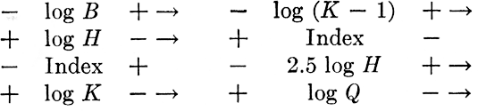
Step 5. Since the indices are fixed at the end of the slide, the position of the scales along their axes must be determined by solving an example and gluing the scales so that they satisfy this location of the index.
Step 6. Place the information contained in the figure title on the back of the rule.
The slide rule, Fig. 6.13, is equivalent to a middle-support rule with the stationary middle-support scale in the groove. This form of rule is satisfactory for equations in which the transfer lines run from one logarithmic scale to another. On the middle-support rule where the transfer lines run from a uniform scale to a logarithmic scale, the diagonal transfer lines must sometimes be followed for a long distance, Which would be difficult if the scale were in the groove of a slip-gage rule.
The slip-gage rule is peculiar in that it apparently has no index marks, but from a consideration of the method of operation it is evident that the end of the slide is an index pointing to the scales in the groove.
6.10. Construction Suggestions. Suitable slide-rule blanks are not easily obtained because of the limited demand for them. Very satisfactory blanks can be constructed by gluing together several layers of cardboard and forming the tongues and grooves by varying the widths of the strips.
All of the special slide rules shown here have been made by gluing paper scales on blanks constructed of Wood. The blanks are 14 in. in length. These rules Work satisfactorily if well-seasoned wood is used and if they are not subjected to extremes of temperature and humidity.
In affixing the scales it is usually better to prepare the scales and then fasten them to the slide-rule blank. The disadvantages of this method are that it is difficult to glue the scales in exactly the right place, as they must be for slide rules without an index, and that the paper on which the scales are constructed changes shape when the glue is applied. On the other hand, if the scales are fastened on the rule first, it is awkward to mark the scales, and if a mistake is made, it is sometimes necessary to glue on new scales and start over again.
It is desirable to apply the glue to the slide-rule blank only, when attaching the scales, and then press the scale in place. A weight of some sort should be placed on the scale until it is dry. Also, the slide and frame should be taken apart for gluing the scales.