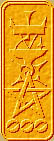
An equation like A + B = SUM requires three scales, but is still very simple:
This is called a Parallel-scale chart. It performs the stunning mathematical feat of adding two numbers. The three scale are parallel (duh.). The origin on all three scales are aligned. In this nomogram, the imaginary line connecting the origins is perpendicular to the scales but this is not required. As long as the three origins are on the same line the nomogram will work. There is one scale for each of the three variables in the equation: A, B, and SUM. The spacing of the strokes on the SUM scale is half the size of the stroke spacing on the other two.
For this nomogram in particular the distance between scale A to scale Sum is the same as the distance between scale B and scale Sum, this is not necessarily true of all parallel scale charts. It depends on the details of the equation the nomogram solves for. This will be explained in the next page.
The red line is the straight-edge (the technical term is Isopleth or Index Line). If you wanted to know the answer to 5 + (-1) = ?, you lay the straight-edge from the 5 on the A scale to the -1 on the B scale, and note the answer where the straight-edge crosses the SUM scale at 4. This is how to use the nomogram to add two numbers.
Alternatively, if you wanted to know what to add to 5 in order to have a sum of 4 (5 - 4 = ?), you'd lay the straight-edge from the 5 on the A scale to the 4 on the SUM scale, and read the answer -1 on the B scale. This is how to use the nomogram to subtract two numbers.
In other words, with a three variable nomogram, given the values of any two variables you can determine the value of the unknown third variable. This is true of all nomograms, they can solve for one unknown given all the other values.
Parallel scale nomograms are used for equations of the form f(a) + f(b) + f(c) = 0. In this most basic of cases, a+b=c becomes a+b-c=0 when converted to match the parallel scale equation form (i.e., re-arranged so there is a zero at the end).
To draw our simple addition nomogram, the equations for scale A are -1 = x and A = y, scale B are 1 = x and B = y, and scale C are 0 = x and 0.5 * C = y. (the last equation is actually -0.5 * -C = y but don't worry about that just yet)
Multiply each y value by your chosen functional modulus μ and you can plot the scales on a piece of graph paper.
Of course, when creating a more complicated parallel scale nomogram, the equations are more involved. Again, this will be explained in the next page.
I'm not going to attempt to explain Logarithms to you. But there is one trick they can do.
If you take two numbers A and B, convert them into logarithms, add the logarithms, then convert the result back into a number, you will get A * B. In other words: adding logarithms is the same as multiplying numbers. This is how slide rules work.
Back in the days of yore before the invention of pocket calculators, books of logarithms were popular. It is far easier and less prone to error to multiply huge numbers by adding logarithms rather than doing it longhand.
What does this have to do with our three line nomogram? If the tick marks are separated by intervals that are logarithmic instead of equal like we have been doing, the result will be a nomogram that does multiplication instead of addition! By the same token it will do division instead of subtraction.
The equation will be log(A)+log(B)-log(C)=0, obviously.
Here is a table done on a spreadsheet. The first row is the numbers on the tick marks of the A and B scales. The second row is the logarithm of the numbers. I decided that I wanted the lines to be 200 millimeters long which means the functional modulus is 200 ( μ = 200/(1.000-0.000) ). The last row is each logarithm multiplied by μ.
| A or B | 1 | 2 | 3 | 4 | 5 | 6 | 7 | 8 | 9 | 10 |
| log(A) | 0.000 | 0.301 | 0.477 | 0.602 | 0.699 | 0.778 | 0.845 | 0.903 | 0.954 | 1.000 |
| *μ | 0 | 60 | 95 | 120 | 140 | 156 | 169 | 181 | 191 | 200 |
| C | 1 | 2 | 3 | 4 | 5 | 6 | 7 | 8 | 9 | 10 | 20 | 30 | 40 | 50 | 60 | 70 | 80 | 90 | 100 |
| log(C) | 0.000 | 0.301 | 0.477 | 0.602 | 0.699 | 0.778 | 0.845 | 0.903 | 0.954 | 1.000 | 1.301 | 1.477 | 1.602 | 1.699 | 1.778 | 1.845 | 1.903 | 1.954 | 2.000 |
| *0.5 | 0.000 | 0.151 | 0.239 | 0.301 | 0.349 | 0.389 | 0.423 | 0.452 | 0.477 | 0.500 | 0.651 | 0.739 | 0.801 | 0.849 | 0.889 | 0.923 | 0.952 | 0.977 | 1.000 |
| *μ | 0 | 30 | 48 | 60 | 70 | 78 | 85 | 90 | 95 | 100 | 130 | 148 | 160 | 170 | 178 | 185 | 190 | 195 | 200 |
For complicated reasons, the origin of a logarithmic scale starts at one, not zero. To draw the scale, simply look at the entry at the bottom row of the above table, measure that many millimeters from the origin, make the tick mark and label with the top row number (e.g. label the tick mark at 156 mm with "6").